Slope Fields and Euler's Method
Objective
In this activity, you'll use Sketchpad to generate a numerical solution to a differential equation, using Euler's method. Euler's method involves a three-step process:
- Choose a starting point.
- Find the tangent to the solution at that point. (Evaluating the differential equation at the current location gives the slope of the tangent.)
- From the starting point, follow the tangent line for a short interval. The point at which you end up is your new starting point, and you begin the process over.
You'll first use a script tool to do these steps, clicking the tool once for each iteration of Euler's method. Once you've traced a number of iterations of a numeric solution, you'll vary both the initial conditions and the differential equation itself, observing the effect on the solution. Finally, you'll use an automated process to generate many more iterations, and observe the effect of changing the iteration interval size on the stability and accuracy of Euler's method.
Steps:
Step 1: Open the file Slopefld.gsp in the Slopefld folder, and observe the slope field for the differential equation dy/dx = ax/y. Drag the slider labeled a to change the parameter and look at slope fields corresponding to an entire family of differential equations.
Step 2: Choose some arbitrary value of a, and change your script tool folder to the Slopefld folder. Click and hold on the script tool icon, and choose the Single Trace tool. Choose an initial position and click this tool in the sketch.
Step 3: Click the tool again on one of the end points of the segment resulting from the first click. Each time you click the tool, it extends the current trace by a fixed increment.
Step 4: By repeatedly clicking on the end point of your existing trace, extend it until you can get some clear idea of the shape of your graph. You should make at least 20 increments in your trace.
Q1. What shape does the trace generate? ___________________________
________________________________________________________
Step 5: To explore a different solution to this differential equation, choose an initial position that does not lie on the solution you've just generated. Click your tool at this spot in the sketch, and extend your trace in both directions.
Q2. How does this second solution differ from the first? _________________
________________________________________________________
Explore More (Interlude)
Before closing your sketch containing two (approximate) solutions to your differential equation, try changing the initial conditions by using the Selection Arrow tool to drag one of the initial points. (This can be a bit tricky, since you've generated additional points that are almost exactly coincident with your original point. To overcome this problem, you can hide any point you select that turns out not to be the correct one.)
As you drag the initial point, observe the behavior of your constructed trace. Can you make it misbehave anywhere? If so, describe where, and see if you can explain the misbehavior.
(Hint: each time you clicked the trace tool in the sketch, it created a segment with two endpoints. You chose only one of those endpoints for the next step of the iteration.)
Steps:
Step 6: Close your sketch without saving, or save it with a different name if you want to keep it.
You'll again trace a solution by numeric methods, but this time you'll use a recursive script that is capable of tracing many steps at a time.
Step 7: Again open the file slopefld.gsp. Click and hold on the script tool icon, and select the Multi-Trace tool. Choose an initial position and click this tool in the sketch.

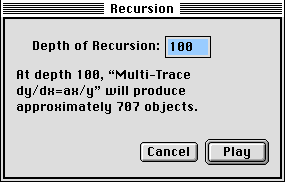
Step 8: A dialog appears asking you to choose the depth to which you want to play the tool. Choose a number that is large enough to see a reasonable amount of the solution, but not so large that your computer is too slow at performing the needed calculations. (Your teacher can probably give you a range within which to choose.)
Step 9: After the trace appears, drag the initial point to a number of new positions, and watch the effect on the solution.
Q3. Describe the resulting shapes: ________________________________
________________________________________________________
The numeric method used results in some inaccuracy in the trace.
Q4. Can you see any evidence of such inaccuracy? Describe: _______________
________________________________________________________
Step 10: Drag slider d to make the step size larger. Observe how this change affects the shape of the traced solution.
Q5. Describe how a larger value of d changes the shape of your trace. Does it make the solution more or less accurate?
________________________________________________________
________________________________________________________
Step 11: Drag d to make the step size smaller. Observe how this change affects the shape of the traced solution.
Q6. Describe how a smaller value of d changes the shape of your trace. Does it make the solution more or less accurate?
________________________________________________________
________________________________________________________
Step 12: Vary the differential equation itself by moving the a slider. For each new value of a, drag the initial point around on the sketch to look at different members of the family of solutions. Try this for several different values of a, being sure to include both positive and negative values.
Q7. When a < 0, how does the shape depend on the value of a? Describe the differences you observe in the shape when the absolute value of a is large, compared to when it's small.
________________________________________________________
________________________________________________________
________________________________________________________
Q8. When you change a from negative to positive, how does the shape of the solutions change?
________________________________________________________
________________________________________________________
________________________________________________________
Q9. When a is positive, investigate the way the solution depends on the initial position. Try initial positions near the x-axis, and try positions near the y-axis. How do the solutions differ in these two situations?
________________________________________________________
________________________________________________________
________________________________________________________