Exploración, Visualización, y Demonstración: La Enseñanza de las Matemáticas con El Geómetra

Conferencia Especial CE-013
Reunion Latinoamericana de Matematica Educativa

Homero Flores, Colegio de Ciencias y Humanidades, Universidad Autonome de Mexico, Mexico, D.F.
Scott Steketee, KCP Technologies, Inc.
Summer 2003

This commentary on the sketch is in English, although the talk itself was delivered in Spanish. The sketch is available in two forms: the initial form (as it appeared at the beginning of the presentation) and the final form (with the various activities completed and, in some cases, with presentation buttons).

1 & 2. Titulos (Title Screens)

We would like to show you several examples of the way in which El Geómetra (in English, The Geometer’s Sketchpad) can be used in demonstrations and in student activities in order to develop student understanding that is more significant and longer lasting. These examples will come from several different areas of mathematics, including Euclidean geometry, transformational geometry, algebra and the study of functions, graphing of functions in Cartesian and polar coordinates, and calculus (including derivatives, anti-derivatives, and integrals). If we had time, we would also show you examples from trigonometry, conic sections, and other areas of mathematics.

As we look at the examples, please remember that they are chosen to show you the features and benefits of the software. When the program is used for demonstration in the classroom, or when it is used by students for direct investigation, the presentation and the examples themselves will be different, and will be adapted to the level and ability of the class.

The first example comes from Euclidean geometry.

3. Centroide (Centroid)

We begin with a blank screen and the tools of Euclidean geometry: the straightedge and compass. We first use the straightedge to construct a triangle. The result is not just a single triangle, but by dragging the vertices it can be transformed into any possible triangle—acute, obtuse, isosceles, right, and so forth.

Next we construct the midpoints of one side. Because we are very strict, we require students to use the compass to construct this first midpoint. But once they have constructed the first, we allow them to use the Midpoint command to construct the other two midpoints. We then use the straightedge again to construct the three medians.

Students will notice that the third median passes through the intersection of the first two medians. On pencil and paper, this would be an observation of only a single case—provided the student had done the construction carefully enough. But with Sketchpad, the student can now transform the result to observe that the statement is true, not just for a single example, but for many differently shaped triangles.

Similarly, the student can now measure two distances from the centroid—to one vertex and to the midpoint on the opposite side—and discover that even when the distances change, there is something constant about the relationship. In a particular configuration, we find that one distance appears to be twice the other. With Sketchpad, we can discover that this relationship holds no matter what the size or shape of the triangle.

To continue our investigation, we can also construct two of the interior triangles and measure their areas. We observe that the areas remain the same, even though the shapes of the two small triangles are very different.

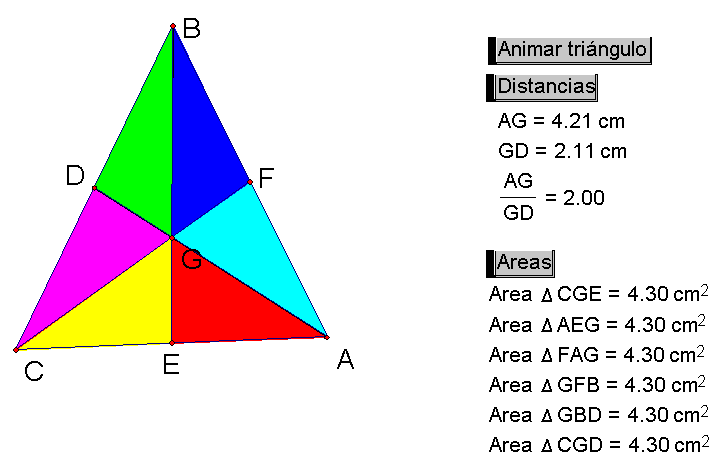
Finally, if we want to allow others to see the results of our work on the Web, we can save our result as a Web page, and put it onto our Web site for all the world to see. We change the size of the sketch to match the size we want to appear on our Web page. Then save the sketch, but instead of saving normally we save it as “html.” When the sketch has been saved, we can open it in a Web browser to see the result.

Most of the constructions you can do in Sketchpad can be saved in this way, but I must tell you that there are some constructions that cannot be saved at this time. Fortunately, all the constructions in this sketch we have just completed can be saved. We will add support for the remaining constructions as we continue to improve Sketchpad version 4.

Next we proceed to an example that involves transformational geometry.

4. Exterior (Exterior Angles)

This is an example of how valuable the combination of Sketchpad and transformational geometry can be. In this example, we are asking students to try to figure out what will be the sum of the exterior angles of a pentagon. To make it easy to see the exterior angles, we will use the ray tool to make the pentagon. [Complete the pentagon.] Now we have five exterior angles, and we could measure them and have Sketchpad add them up. But we will take a different approach.

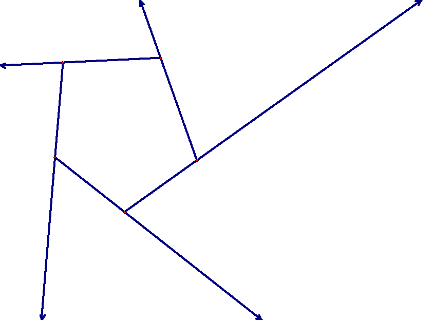
First we mark one vertex as the center. This vertex serves as the center for either rotation or dilation. In order to rotate objects, we can make use of Sketchpad’s rotation Arrow tool. If we rotate the remaining vertices about the center, we notice that the angles do not change. Similarly, if we use the Dilation Arrow tool to dilate the remaining vertices, we notice that the angles still do not change. Now let’s think one more time about the original question: what is the sum of the exterior angles of the polygon? [Shrink the polygon to a point, so the exterior angles emanate from a single point.]

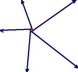
Here is an instance where the student can not only give the correct answer, but will immediately know that this is the correct answer not only for a pentagon, but for any possible simple convex polygon. In addition, the nature of the demonstration is such that the student will remember this for a very long time—he or she can always remember what it will look like if the polygon is shrunk to a single point.

Next we go on to an example from algebra involving operations on integers.

5. Multiplica (Multiplication on the number line)

In this example we have a magic machine that takes two numbers as input and produces some output. Students don’t need to know exactly how the machine works, but they can see first that it produces exactly the results they normally get when they multiply two positive numbers.

Then we watch how the machine behaves when we multiply a positive number by a negative number, and we see that the behavior of the machine is consistent. The movement of the result is continuous as one of the numbers crosses zero and becomes negative.

Finally, we ask students what they expect the machine to do when both numbers are negative. If the machine behaves continuously, what will happen as the second number crosses zero?

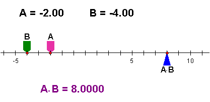
This machine makes it very easy for a student to see one argument, by continuity, for why it is that the product of two negative numbers is positive.

Now we proceed to an algebra sketch that illustrates the concept of a function.

6. Dina 1 (Dynagraph 1)

In this example, we have four different functions, presented on four pairs of axes. First, please look at the first function. We can change the input to the function in any way we want on the input axis, and the output is displayed on the output axis. This allows us to investigate the behavior of a function without ever talking about numbers, but instead thinking only about input and output. Not only this, but we can use this method for developing other concepts such as the composition of functions.

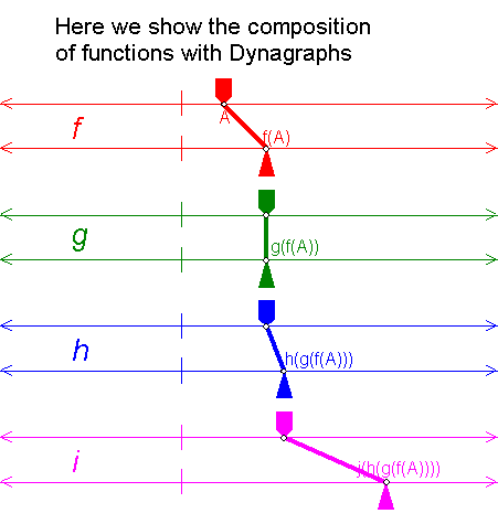
For instance, to compose functions f and j, we first remove the other functions so they will not be in the way. Then we split the input of j from its input axis, and instead attach it to the output of f. This creates the composition of functions f and j.

7. Dina 2 (Dynagraph 2)

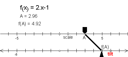
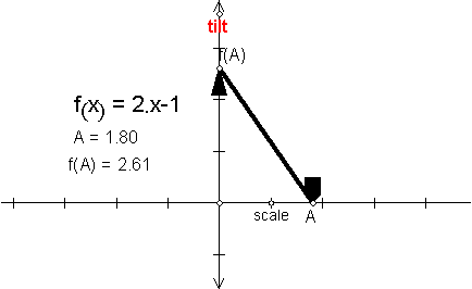
In this example, we move from the previous representation, using parallel axes for input and output, to the Cartesian representation, using perpendicular axes. We first explore how the representations are equivalent in meaning though they differ in form. We then construct perpendiculars, and the intersection of the perpendiculars, so that we can see a traditional graph on the x-y axes.

8. Familia (Family of functions)

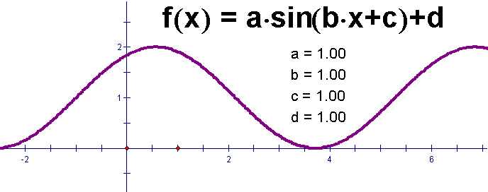
It is very easy to graph a function using Sketchpad. Choose Plot New Function from the Graph menu, and type in the function, in this case sin(x). Sketchpad asks us whether we want to graph the sine function using degrees or radians. We choose radians, and the graph appears.

If this is all that Sketchpad can do, we should use a graphing calculator and not a computer. But we can graph an entire family of functions by adding a parameter to our function. We choose New Parameter from the Graph menu, and name the new parameter “a.” We do it again and name the second parameter “b.” Now we can double-click to edit our function, and change the function to one that uses the parameters.

There is no change yet after editing, because both parameters have the value one. We can change the values of the parameters by pressing the “+” and “-“ keys on the keyboard, to explore this family of functions. We can easily look at particular values for either parameter by double-clicking the parameter and typing a new value. We can also animate the parameters to watch the function and the graph change quickly.

9. Polar (Polar Functions)

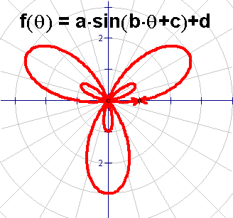
Just as we can graph a family of functions using rectangular coordinates, we can also use polar coordinates. In this example we have already graphed a function, and if we show the controls you can see that the value of b is 1. Let us change the value of b to 3 to see the results. We like this sketch a lot, because when we animate parameter c we can imagine we are the pilot of an airplane about to take off from the airport.

The next group of examples comes from the area of calculus.

10. Derivada (Derivative)

In this example we combine several different activities to help students understand the concept and the definition of a derivative. We would not do this entire activity at one time, but would do half of it one day, let the students think about it, and do the other half on a different day.

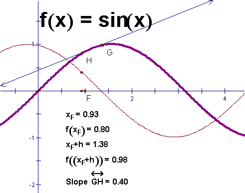
For the first part of the activity we start with a function, for instance sin(x). We then use the line tool to construct a secant line.

Notice that we can drag this secant line back and forth along the function, and we can also animate it so that it goes back and forth automatically.

Now that we have a secant line, we want to study the “slope function.” In other words, we want to observe the behavior of the slope of the secant line at different positions on the function. We measure the slope, and also measure the x-value for one of the end points. We can plot the point that shows the slope, and trace this point. When the secant line moves now, we can observe the slope function for the secant line.

However, the slope of the secant is not an accurate result for the slope of the function itself. We can make the result much more accurate if we move the two points A and B very close together. Now we will see a much better approximation of the value of the slope function.

On a later day we would do a second activity. In this second activity we place a point on the x-axis and measure its x-value. We then calculate the corresponding value of f(x). If we plot these two values, we have one point on the function.

This time we want to control the separation of the two points, so we make a parameter h. We set the properties of this parameter so that it can change by very small values—0.01 every time we press the “+” or “-” key.

If we calculate both the value of x + h and of f(x + h), we will have the required coordinates for a second point on the function. We can now use these two points to construct a secant line. This line is different from the previous activity in an important way, because we can now control the separation of the two points very precisely.

Let us again measure the slope of the secant line, and then plot the value of the slope as a function of x. We can even plot the locus of the plotted point for different values of x, to see the entire slope function at one time. And we can change the separation of the two points, to make the result more accurate or less accurate for the slope of the tangent. And we can also see why it is that we may let the value of h approach zero, but we must never let h actually be equal to zero.

11. Antiderivada (Antiderivative)

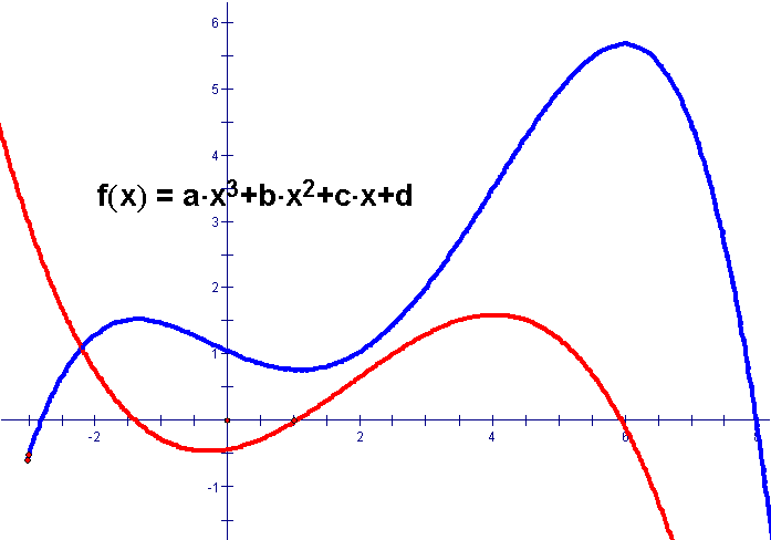
In this next example we reverse the idea of a derivative. Here the student already has the graph of the derivative, but does not know what the graph of the original function looks like. There are two parts to this activity also: to trace the antiderivative by hand, and then to trace automatically.

To trace the antiderivative by hand, the student shows the probe, and then has to use the mouse to drag point P in the correct direction. You can see what happens when we go the correct way, and you can also see what happens when we go the incorrect way. Let us start again and try to do it correctly. The student will have to make several tries before getting a good result. The student should also try this method using several different functions. The resulting approximation is not exact, but the process of using the mouse to follow the probe is a very good way for the student to begin to understand the principle behind Euler’s method.

To trace the antiderivative automatically, we will erase the traces and stop the segment from being traced. Then we tell Sketchpad to iterate the probe by constructing a new probe that starts where the original probe finishes. We use the Iterate command on the Transform menu to do this. When Sketchpad creates the iteration, it originally makes only three iterations. We can use the Properties dialog box to say how many iterations we want; in this case we will make 1000.

Now we can see what the effect will be if we change the size of our probe, so that we get more accurate results with a smaller step size, and less accurate results with a larger step size. We can also change our initial conditions, in order to see the effect on the approximate solution.

We will not try to show you today an activity for the Fundamental Theorem of Calculus, but we will show you a quick example, already constructed, of demonstrating the Definite Integral with Sketchpad.

12. Integral (Definite Integral)

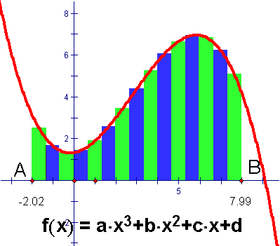
In this sketch we use rectangles to approximate the area under the graph. Here the height of the rectangle is determined by the value of the function at the midpoint of the integral. We can easily change the limits of the integration. We could also change the function itself if we want to.

But most interesting to observe is the result of changing the number of intervals. We can do this by hand if we want. It is especially interesting to watch as Sketchpad animates the value of n.

We could do much more with calculus if we had the time, exploring the fundamental theorem of calculus and also doing activities with slope fields. But instead we will show you two more quick examples from other areas, one from math and one from physics. The first is a fractal called the Sierpinski triangle.

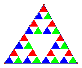
13. Fractales (Fractals—Sierpinski Triangle)

This famous fractal is very easy to construct using the new Iteration command in Sketchpad Version 4. After we have constructed it, we can change the depth and watch how the fractal appearance changes.

Our final example is from the area of physics.

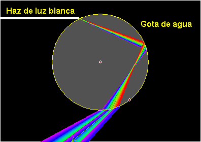
14. Ciencia (Science: Rainbow)

In this example, we have used Sketchpad to show the result of a ray of light from the sun reflecting inside a drop of water. The colors result when the ray of light bends as it enters the drop of water and as it leaves the drop of water. We can see what the angles are for the different colors depending on  exactly where the ray of light enters the drop. The results of this sketch can help the physics student understand how a rainbow is formed.

Back to Recent Talks